Examples

Wavelet functions

The example is located in examples/wavelet_fun.py.

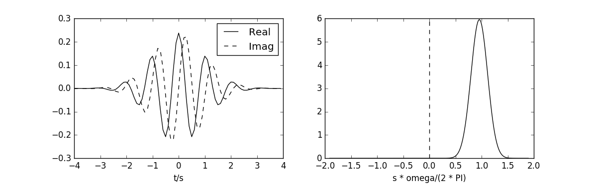
# This code reproduces the figure 2a in (Torrence, 1998).
# The plot on the left give the real part (solid) and the imaginary part
# (dashed) for the Morlet wavelet in the time domain. The plot on the right
# give the corresponding wavelet in the frequency domain.
# Change the wavelet function in order to obtain the figures 2b 2c and 2d.

from __future__ import division

import numpy as np
import scipy as sp
import matplotlib.pyplot as plt

import cwave


wavelet = cwave.Morlet() # Paul(), DOG() or DOG(m=6)
dt = 1
scale = 10*dt
t = np.arange(-40, 40, dt)
omega = np.arange(-1.2, 1.2, 0.01)

psi = wavelet.time(t, scale=scale, dt=dt)
psi_real = np.real(psi)
psi_imag = np.imag(psi)
psi_hat = wavelet.freq(omega, scale=scale, dt=dt)

fig = plt.figure(1)

ax1 = plt.subplot(121)
plt.plot(t/scale, psi_real, "k", label=("Real"))
plt.plot(t/scale, psi_imag, "k--", label=("Imag"))
plt.xlabel("t/s")
plt.legend()

ax2 = plt.subplot(122)
plt.plot((scale*omega)/(2*np.pi), psi_hat, "k")
plt.vlines(0, psi_hat.min(), psi_hat.max(), linestyles="dashed")
plt.xlabel("s * omega/(2 * PI)")

plt.show()

Nino3 SST time series

The example is located in examples/nino.py.

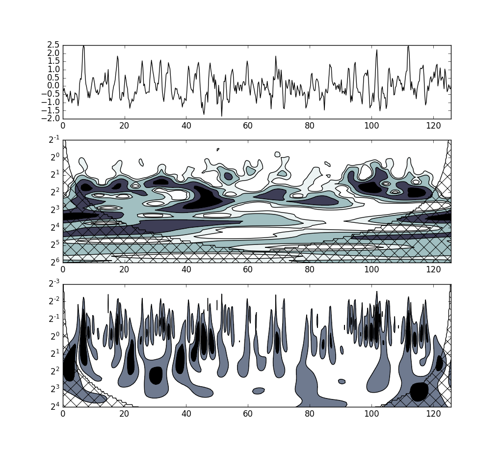
# This code reproduces the figure 1a in (Torrence, 1998).
# This example does not include the zero padding at the end of the series and
# the red noise analysis.

from __future__ import division

import numpy as np
import scipy as sp
import matplotlib.pyplot as plt
import matplotlib.gridspec as gridspec

import cwave

dt = 0.25
dj = 0.125

x = np.loadtxt("sst_nino3.txt")
s = cwave.Series(x, dt)

var = np.var(s.x)
N = s.x.shape[0]
times = dt * np.arange(N)

## Morlet
w_morlet = cwave.Morlet()
T_morlet = cwave.cwt(s, w_morlet, dj=dj, scale0=2*dt)
Sn_morlet= T_morlet.S() / var
# COI
taus_morlet= [T_morlet.wavelet.efolding_time(scale) for scale in T_morlet.scales]
mask_morlet = np.zeros_like(T_morlet.W, dtype=np.bool)
for i in range(mask_morlet.shape[0]):
    w = times < taus_morlet[i]
    mask_morlet[i, w] = True
    mask_morlet[i, w[::-1]] = True

## DOG
w_dog = cwave.DOG()
T_dog = cwave.cwt(s, w_dog, dj=dj, scale0=dt/2)
Sn_dog = T_dog.S() / var
# COI
taus_dog= [T_dog.wavelet.efolding_time(scale) for scale in T_dog.scales]
mask_dog = np.zeros_like(T_dog.W, dtype=np.bool)
for i in range(mask_dog.shape[0]):
    w = times < taus_dog[i]
    mask_dog[i, w] = True
    mask_dog[i, w[::-1]] = True

## Plot

fig = plt.figure(1)
gs = gridspec.GridSpec(3, 1, height_ratios=[0.6, 1, 1])

# plot the series s
ax1 = plt.subplot(gs[0])
p1 = ax1.plot(times, s.x, "k")

# plot the wavelet power spectrum (Morlet)
ax2 = plt.subplot(gs[1], sharex=ax1)
X, Y =  np.meshgrid(times, T_morlet.scales)
plt.contourf(X, Y, Sn_morlet, [1, 2, 5, 10], origin='upper', cmap=plt.cm.bone_r,
    extend='both')
plt.contour(X, Y, Sn_morlet, [1, 2, 5, 10], colors='k', linewidths=1, origin='upper')

# plot COI (Morlet)
plt.contour(X, Y, mask_morlet, [0, 1], colors='k', linewidths=1, origin='upper')
plt.contourf(X, Y, mask_morlet, [0, 1], colors='none', origin='upper', extend='both', 
    hatches=[None, 'x'])
ax2.set_yscale('log', basey=2)
plt.ylim(0.5, 64)
plt.gca().invert_yaxis()

# plot the wavelet power spectrum (DOG)
ax3 = plt.subplot(gs[2], sharex=ax1)
X, Y =  np.meshgrid(times, T_dog.scales)
plt.contourf(X, Y, Sn_dog, [2, 10], origin='upper', cmap=plt.cm.bone_r,
    extend='both')
plt.contour(X, Y, Sn_dog, [2, 10], colors='k', linewidths=1, origin='upper')

# plot COI (DOG)
plt.contour(X, Y, mask_dog, [0, 1], colors='k', linewidths=1, origin='upper')
plt.contourf(X, Y, mask_dog, [0, 1], colors='none', origin='upper', extend='both', 
    hatches=[None, 'x'])
ax3.set_yscale('log', basey=2)
plt.ylim(0.125, 16)
plt.gca().invert_yaxis()

plt.show()

Filtering

TODO